Fairness
notation, definitions, data, legality
THIS IS AN OLD DRAFT
SEE THE NEW ONE HERE
A very narrow goal: Understand the mathematical definitions of quantitative “fairness” from the literature by writing them in common notation in one place.
A broader goal: Understand what assumptions each notion of “fairness” is making (e.g. about the data). Ask what it means for an algorithm to be “fair” when it is one component of a system that in its totality is massively unequal. Ask what assumptions underlie the formulation as a constrained optimization problem in which fairness is a constraint on some desirable (by whom?) maximization.
We focus on the criminal justice context for concreteness, but also consider the related topic of health disparities.
Notation
$Y =$ outcome, for simplicity only binary (e.g. arrest, a mismeasurement of offense)
$A =$ race, for simplicity only $ = b$ or $w$
$X =$ observed covariates (excludes $A$)
$S = \hat{P}(Y = 1 | A, X) =$ estimated probability of the outcome
$= f(A, X, \mathbf{Y}^{\textrm{train}}, \mathbf{A}^{\textrm{train}}, \mathbf{X}^{\textrm{train}})$ where $f$ can be stochastic and takes training data
$d =$ decision/classifier, e.g. $=I(S > t)$ where $t =$ cutoff/threshold. More generally,
$= f_d(A, X, \mathbf{Y}^{\textrm{train}}, \mathbf{A}^{\textrm{train}}, \mathbf{X}^{\textrm{train}})$ where $f_d$ can be stochastic and takes training data
(Some papers aren’t clear whether they mean $S$ or $d$)
$d(b) =$ decision had the person been black (a counterfactual or potential outcome, see challenges with causal interpretations of race)
$d(w) =$ decision had the person been white
The observed $d = d(b)$ if the person is black and $= d(w)$ if the person is white. We can also define potential outcomes for $S$.
Index people by $i,j$, e.g. $Y_i$ is the outcome for person $i$. Imagine drawing people (independently and identically) from a population distribution $p(Y,A,X,S,S(b),S(w),d,d(b),d(w) | \mathbf{Y}^{\textrm{train}}, \mathbf{A}^{\textrm{train}}, \mathbf{X}^{\textrm{train}})$. Many fairness definitions are properties of this distribution. From now on we assume everything is conditional on the training data.
Definitions
Here are definitions of fairness found in the literature, along with some results related to them. We link to papers using the definition or making the claim. Context buttons (which need work!) provide intuition and results for widely-used tools like COMPAS.
Definitions based on $p(Y, A, S)$
- Calibration:
$P(Y = 1 | S = s, A = b) = P(Y = 1 | S = s, A = w)$ [Chouldechova]
(Hardt et al. call this matching conditional frequencies)
Strong calibration: also requires $= s$ [Kleinberg et al.]
$S = P(Y = 1 | A, X) \Rightarrow$ strong calibration (but not the reverse)
Proof: As in exercise 37 on p.417 of Blitzstein and Hwang,
$E(Y | S, A) \overset{\textrm{iterate over }X}{=} E(E(Y | S, A, X) | S, A) \overset{S=S(A,X)}{=} E(E(Y | A, X) | S, A) \overset{\textrm{assumption that }S = E(Y | A, X)}{=} S$
$E(Y | S) \overset{\textrm{iterate over }A,X}{=} E(E(Y | S, A, X) | S) \overset{S=S(A,X)}{=} E(E(Y | A, X) | S) \overset{\textrm{assumption that }S = E(Y | A, X)}{=} S$
This proof works with any $X$ (including no $X$). See below about redlining.
- Balance for the negative class:
$E(S | Y = 0, A = b) = E(S | Y = 0 , A = w)$ [Kleinberg et al.]
- Balance for the positive class:
$E(S | Y = 1, A = b) = E(S | Y = 1 , A = w)$ [Kleinberg et al.]
Cannot have 1 + 2 + 3 unless $S=Y$ (perfect prediction) or $P(Y=1|A=b) = P(Y=1|A=w)$ (equal base rates) [Kleinberg et al.]
Definitions based on $p(Y, A, d)$
The next four definitions come from the four margins of the Confusion Matrix:
| Prevalence | ||||
|---|---|---|---|---|
| $Y=1$ | $Y=0$ | “base rate” | ||
| $P(Y=1)$ | ||||
| Positive Predictive Value | False Discovery Rate | |||
| $d=1$ | True Positive | False Positive | (PPV) | (FDR) |
| (TP) | (FP) | $P(Y = 1 | d = 1)$ | $P(Y = 0 | d = 1)$ | |
| False Omission Rate | Negative Predictive Value | |||
| $d=0$ | False Negative | True Negative | (FOR) | (NPV) |
| (FN) | (TN) | $P(Y = 1 | d = 0)$ | $P(Y = 0 | d = 0)$ | |
| True Positive Rate | False Positive Rate | |||
| (TPR) | (FPR) | Accuracy | ||
| $P(d = 1 | Y = 1)$ | $P(d = 1 | Y = 0)$ | $P(d = Y)$ | ||
| False Negative Rate | True Negative Rate | |||
| (FNR) | (TNR) | |||
| $P(d = 0 | Y = 1)$ | $P(d = 0 | Y = 0)$ |
those given special names have citations:
- equal NPVs: $P(Y=0 | d = 0, A = b) = P(Y=0 | d = 0, A = w)$
$\Leftrightarrow$ equal FORs: $P(Y=1 | d = 0, A = b) = P(Y=1 | d = 0, A = w)$
$\Leftrightarrow Y \perp A | d = 0$
- Predictive parity (equal PPVs): $P(Y=1 | d = 1, A = b) = P(Y=1 | d = 1, A = w)$ [Chouldechova]
$\Leftrightarrow$ equal FDRs: $P(Y=0 | d = 1, A = b) = P(Y=0 | d = 1, A = w)$
$\Leftrightarrow Y \perp A | d = 1$
(Simoiu et al. describe assessing equal PPVs as “outcome tests”.)
- Error rate balance (equal FPRs): $P(d = 1 | Y = 0, A = b) = P(d = 1 | Y = 0, A = w)$ [Chouldechova]
$\Leftrightarrow$ equal TNRs: $P(d = 0 | Y = 0, A = b) = P(d = 0 | Y = 0, A = w)$
$\Leftrightarrow d \perp A | Y = 0$
- Error rate balance (equal FNRs): $P(d = 0 | Y = 1, A = b) = P(d = 0 | Y = 1, A = w)$ [Chouldechova]
$\Leftrightarrow$ Equal opportunity (equal TPRs): $P(d = 1 | Y = 1, A = b) = P(d = 1 | Y = 1, A = w)$ [Hardt et al., Kusner et al.]
$\Leftrightarrow d \perp A | Y = 1$
Cannot have 5 + 6 + 7 unless $d=Y$ (perfect prediction) or $P(Y=1|A=b) = P(Y=1|A=w)$ (equal base rates) because $\textrm{FPR} = \frac{p}{1-p} \frac{1-\textrm{PPV}}{\textrm{PPV}} (1 - \textrm{FNR})$ [Chouldechova]
4+5. Conditional use accuracy equality: $Y \perp A | d$ [Berk et al.]
6+7. Equalized odds [Hardt et al.], Conditional procedure accuracy equality [Berk et al.]: $d \perp A | Y$
- Statistical/Demographic parity: $P(d = 1 | A = b) = P(d = 1 | A = w)$ [Chouldechova, Kusner et al.]
or $E(S | A = b) = E(S | A = w)$ [Kleinberg et al.]
Conditional statistical parity: $P(d = 1 | L = l, A = b) = P(d = 1 | L = l, A = w)$, for legitimate factors $L$ [Corbett-Davies et al.]
(Kamiran et al. call this conditional non-discrimination.)
(Simoiu et al. describe assessing parity as “benchmarking”.)
- Overall accuracy equality: $P(d = Y | A = b) = P(d = Y | A = w)$ [Berk et al.]
- Treatment equality (equal FN/FP): $\frac{P(d=0, Y=1 | A = b)}{P(d=1, Y=0 | A = b)} = \frac{P(d=0, Y=1 | A = w)}{P(d=1, Y=0 | A = w)}$ [Berk et al.]
Definitions that do not marginalize over $X$ (“individual” definitions)
aaronsadventures describes how the above definitions can hide a lot of sins by marginalizing (i.e. averaging) over $X$. For example, suppose an algorithm gives $d = 1$ if and only if either $A = b$ and $X = 1$ or $A = w$ and $X = 0$. By the law of total probability:
So if $P(X = 1 | A = b) = P(X = 0 | A = w)$ then we satisfy parity. But within strata defined by $X$, we do not:
This is a verson of Simpson’s paradox, see p.67-69 of Blitzstein and Hwang.
As aaronsadventures puts it:
If you know some fact about yourself that makes you think you are not a uniformly random white person, the guarantee can lack bite.
The next definitions consider these facts, i.e. the $X$ variables.
- Fairness through unawareness: $d_i = d_j$ if $X_i = X_j$ (no use of $A$) [Kusner et al.]
A property of $p(d,X)$? Maybe: $\exists f$ such that $p(d|X) = 1$ if $d = f(X)$ and $= 0$ otherwise.
- Individual Fairness: $||d_i - d_j|| \leq \epsilon’$ if $||X_i^{\textrm{true}} - X_j^{\textrm{true}}|| \leq \epsilon$ where we think $X^{\textrm{true}}$ are fair to use for decisions [Friedler et al.]
(Dwork et al. call this the Lipschitz property.)
This is possible if What You See Is What You Get: $\exists$ an observation process $g: X^{\textrm{true}} \rightarrow X$ that doesn’t distort too much, i.e. $\bigg | ||X_i^{\textrm{true}} - X_j^{\textrm{true}}|| - ||g(X_i^{\textrm{true}}) - g(X_j^{\textrm{true}}) ||\bigg | < \delta$
AND
if you use an Individual Fairness Mechanism $\textrm{IFM}: X \rightarrow d$ that doesn’t distort too much, i.e. $\bigg | ||X_i - X_j|| - ||\textrm{IFM}(X_i) - \textrm{IFM}(X_j) ||\bigg | < \delta’$
A property of $p(d,X,X^{\textrm{true}})$?
Which $X$s?
We defined the risk score as $S = \hat{P}(Y = 1 | A, X)$. But what if the risk score does not use (i.e. condition on) all of $X$?
Corbett-Davies et al. give an example where ignoring $X$ for white people helps them because the average across $X$ is below the “high risk” threshold $t$. Conversely, redlining is an example where ignoring $X$ for black people hurts them because the average across $X$ is above the “high risk” threshold $t$. In fact, we don’t have to ignore all of $X$ for this to happen. Consider $X = (X_1, X_2)$:
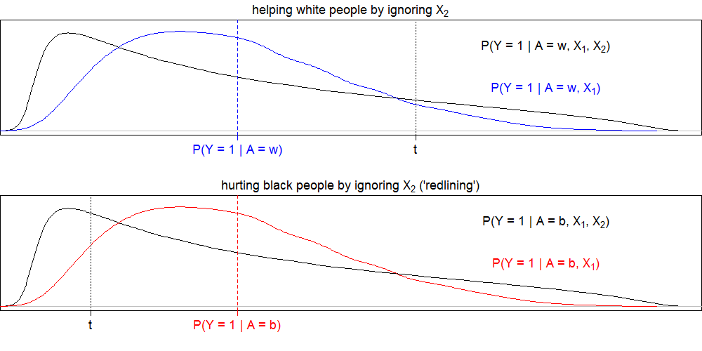 In both cases it is possible to satisfy strong calibration. So we see that strong calibration does not protect against something clearly discriminatory. This motivates a fairness definition from the authors of Corbett-Davies et al., but not in the paper formally:
- Best estimate fairness: $S = S(A,X)$ is fair if there does not exist an easily-obtainable $X’$ and an $S’ = S’(A,X’)$ such that $\textrm{AUC}(S,Y) < \textrm{AUC}(S’,Y)$ where AUC is the area under the receiver operating characteristic curve.
$\Rightarrow$ strong calibration.
Proof: if a score is not strongly calibrated, we proved $\Rightarrow \nexists X$ s.t. $S = P(Y = 1 | A, X)$. This $\overset{*}{\Rightarrow}$ best estimate fairness is not satisfied, since $S = P(Y = 1 | A, X)$ would have a higher AUC.
Definition 13 is not based on any margins of the distribution $p(Y,A,X,S)$ because it allows easily-obtainable new $X’$. But:
- Best estimate fairness given $A$, $X$: $S = S(A,X)$ is fair if there does not exist an $S’ = S’(A,X)$ such that $\textrm{AUC}(S,Y) < \textrm{AUC}(S’,Y)$.
$\overset{*}{\Leftrightarrow} S = P(Y = 1 | A, X)$, which is a property of $p(Y,A,X,S)$. But we have finite training data, so this will not be satisfied exactly.
*: HELP NEEDED - Want to find a proof that for a given $X$, $P(Y = 1 | X)$ has the highest AUC among deterministic functions of $X$…?
- Single threshold fairness: $\exists t$ such that $d = I(S > t)$.
Definition based on $p(S,d)$.
13+15. Corbett-Davies et al. sense of fairness
Corbett-Davies et al. also write:
One might similarly worry that the features x are biased in the sense that factors are not equally predictive across race groups…
This problem could be solved by including $A$ and interactions $A*X$ in the model. But they say:
explicitly including race as an input feature raises legal and policy complications, and as such it is common to simply exclude features with differential predictive power. While perhaps a reasonable strategy in practice, we note that discarding information may inadvertently lead to the redlining effects…
Health disparities - which $X$s?
Broadening from the criminal justice context, consider the related topic of health disparities. Bailey et al. name three pathways from racism to health disparities: residential segregation, health care disparities, and discriminatory incarceration. Focusing on the second, LeCook et al. name three definitions of health care disparities, which differ by choice of $X$. Analogous to our notation, let $d =$ utilization of health care. Consider two sets of $X$ variables: socioeconomic status ($\textrm{SES}$) and health care needs and preferences ($L$). Health care disparities can be defined as:
- Residual direct effect (RDE): $E[d|A=b,\textrm{SES},L] - E[d|A=w,\textrm{SES},L]$
- Unadjusted:
$E[d|A=b] - E[d|A=w]$
Requiring this be 0 is statistical parity. - Institute of Medicine (IOM) definition:
$E[d|A=b,L] - E[d|A=w,L]$ [IOM 2003]
Requiring this be 0 is conditional statistical parity where $L$ are considered legitimate factors.
Causal definitions
Papers that use causal definitions often do not make explicit the difference between $S$ and $d$. Below we write all definitions with $d$ for convenience.
- Fair inference: no unfair path-specific effects (PSEs) of $A$ on $d$ [Nabi and Shpitser]
- Counterfactual fairness: $p(d(b) | A = a, X = x) = p(d(w) | A = a, X = x)$ [Kusner et al.]
To satisfy this, Kusner et al. propose $d$ be a function of non-descendents of $A$, but if arrows in the causal diagram represent individual-level effects, this implies a stronger definition of fairness: $d(b) = d(w)$
- No unresolved discrimination: there is no directed path from $A$ to $d$ unless through a resolving variable [Kilbertus et al.]
Resolving variable: a variable whose influence from $A$ we accept as non-discriminatory (e.g. we decide that it is acceptable for race to affect admission rates through department choice)
- No proxy discrimination: $p(d(a)) = p(d(a’))$ for all $a,a’$ for a proxy variable $A^\textrm{proxy}$ [Kilbertus et al.]
Proxy variable: descendent of $A$ we choose to label as a proxy (e.g. we decide to label skin color as a proxy, and disallow it from affecting admissions)
Causal diagrams.
The causal fairness literature differs on whether $Y$, $d$, or both are included in the causal diagrams. Nabi and Shpitser include $d$ in the causal diagrams. Kusner et al. include $Y$ in the causal diagrams (even though they define fairness in terms of effects on $d$). Kilbertus et al. include both $Y$ and $d$ in the causal diagrams (in their Figure 2 only).Causal interpretation of race.
Above, we defined $d(b)$ as the decision had the person been black and $d(w)$ as the decision had the person been white.
But what does this mean?- What is meant by “black”? “white”?
- Even if we could define these, what is meant by “had the person been black”?
VanderWeele and Robinson propose:
- Decide variables you want to include in “race” (e.g. physical phenotype, cultural context)
- Let $\textrm{SES}$ be family and neighborhood socioeconomic status at conception. Two interpretations of $\beta \equiv E[d|A=b,\textrm{SES}] - E[d|A=w,\textrm{SES}]$:
- With counterfactuals under race
Assume that the effect of $A$ on $d$ is unconfounded conditional on $\textrm{SES}$: $E[d(a)|\textrm{SES}] = E[d|A=a,\textrm{SES}]$.
Then $\beta = E[d(b)-d(w)|\textrm{SES}]$ - Without counterfactuals under race
Let $d(ses)$ be the decision had the person’s $\textrm{SES}$ been set to $ses$.
Assume that the effect of $\textrm{SES}$ on $d$ is unconfounded conditional on $A$: $E[d(ses)|A] = E[d|\textrm{SES}=ses, A]$.
Assume also that $\beta$ doesn’t depend on $\textrm{SES}$.
Then $\beta = E[d(ses_w)|A=b] - E[d|A=w]$
where $ses_w$ is drawn from $p(\textrm{SES} | A = w)$.
This is the racial inequality that would remain if the family and neighborhood socioeconomic status at conception for the black population were set equal to that of the white population.
- With counterfactuals under race
Hernan and Robins introduce counterfactuals as outcomes only under well-defined interventions, see Sections 3.4 (Consistency) and 3.5 (Well-defined interventions are a pre-requisite for causal inference).
In contrast, Pearl 2009 allows counterfactuals under conditions without specifying how those conditions are established, see Section 11.4.5 (Causation without Manipulation!!!).
Greiner and Rubin advocate for a shift in focus from race to perceptions of race, in order to study disparate treatment (as opposed to disparate impact).
Data
It is important to note that $Y, \mathbf{Y}^{\textrm{train}}$ are what is measured (e.g. arrest), which is often different from the $Y^{\textrm{true}}, \mathbf{Y}^{\textrm{true, train}}$ (e.g. offense). Lum highlights this issue, largely overlooked in the literature, which often uses the words “arrest” and “offense/crime” interchangeably (until the discussion section). Corbett-Davies et al. make the distinction in their discussion section:
But arrests are an imperfect proxy. Heavier policing in minority neighborhoods might lead to black defendants being arrested more often than whites who commit the same crime [31 - Lum and Isaac]. Poor outcome data might thus cause one to systematically underestimate the risk posed by white defendants. This concern is mitigated when the outcome $y$ is serious crime — rather than minor offenses — since such incidents are less susceptible to biased observation. In particular, [38 - Skeem and Lowencamp] note that the racial distribution of individuals arrested for violent offenses is in line with the racial distribution of offenders inferred from victim reports and also in line with self-reported offending data.
According to differential selection theory, racial disparities reflect bias in policing and decisions about arrest. This theory applies less to crimes of violence than to (victimless) crimes that involve greater police discretion (e.g., drug use, “public order” crimes; see Piquero and Brame, 2008). For the sake of completeness, we also report results for “any arrest.”
In our view, official records of arrest — particularly for violent offenses — are a valid criterion. First, surveys of victimization yield “essentially the same racial differentials as do official statistics. For example, about 60 percent of robbery victims describe their assailants as black, and about 60 percent of victimization data also consistently show that they fit the official arrest data” (Walsh, 2009, p. 22). Second, self-reported offending data reveal similar race differentials, particularly for serious and violent crimes (see Piquero, 2015).
But Piquero says:
In official (primarily arrest) records, research has historically revealed that minorities (primarily Blacks because of the lack of other race/ethnicity data) are overrepresented in crime, especially serious crimes such as violence. More recently, this conclusion has started to be questioned, as researchers have started to better study and document the potential Hispanic effect. Analyses of self-reported offending data reveal a much more similar set of estimates regarding offending across race, again primarily in Black-White comparisons…
Piquero and Brame use both arrest record and self-report data from a sample of “serious adolescent offenders” in Philadephia and Phoenix. They found little evidence of racial differences in either self-report or arrest record data. But what about datasets that show big racial differences in arrests? For example, ProPublica’s analysis of COMPAS used arrest data from Broward county, Florida. The dataset was used in several subsequent papers as well. It includes racial differences for both general arrests and arrests for alleged violent crimes (see Flores et al. p.12, 14). So I’m not convinced that differential measurement error is not substantial for violent crimes too.
Are there analytical ways around this measurement error issue? In v1 of their paper, Nabi and Shpitser suggested the following:
For instance, recidivism in the United States is defined to be a subsequent arrest, rather than a subsequent conviction. It is well known that certain minority groups in the US are arrested disproportionately, which can certainly bias recidivism risk prediction models to unfairly target those minority groups. We can address this issue in our setting by using a missingness model, a simple version of which is shown in Fig. 1 (d), which is a version of Fig. 1 (a) with two additional variables, $Y(1)$ and $R$. $Y(1)$ represents the underlying true outcome, which is not always observed, $R$ is a missingness indicator, and $Y$ is equal to $Y(1)$ if $R = 1$ and equal to “?” otherwise…Fig. 1 (d) corresponds to a missing at random (MAR) assumption…
They distinguish between arrest and conviction (which is not identical to offense, the true variable of interest, but we ignore this for now). They use $Y$ to denote observed arrests and $Y(1)$ to denote unobserved conviction. The measurement problem is that $Y \ne Y(1)$. Nabi and Shpitser describe an observed indicator $R$ such that when $R = 1$, we have $Y = Y(1)$. Thus, conviction data $Y(1)$ are known for a subset ($R = 1$) of people. Missing at random (MAR)1 assumes $Y(1) | X, R = 1 \overset{\textrm{MAR}}{=} Y(1) | X$, allowing use of known conviction data for valid inference. More generally, we can let $R$ be an indicator for observing convictions, without assuming arrest equals conviction, i.e. $Y = Y(1)$, when $R = 1$. Are any risk tools trained on conviction data? Has anyone done a ProPublica-type analysis with conviction data?
Legality - very rough (need help from lawyers)
U.S. courts have applied strict scrutiny if a law or policy either
- infringes on a fundamental right, or
- uses race, national origin, religion, or alienage.
Strict scrutiny: the law or policy must be
- justified by a compelling government interest,
- narrowly tailored to achieve that goal, and
- the least restrictive means to achieve that goal.
Equal Protection Clause of the Fourteenth Amendment:
All persons born or naturalized in the United States, and subject to the jurisdiction thereof, are citizens of the United States and of the State wherein they reside. No State shall make or enforce any law which shall abridge the privileges or immunities of citizens of the United States; nor shall any State deprive any person of life, liberty, or property, without due process of law; nor deny to any person within its jurisdiction the equal protection of the laws.
Strict scrutiny has been applied in some cases (but not all, e.g. not in gender cases) that involve the Equal Protection Clause. Strict scrutiny is also applied in some cases that involve Free Speech.
The first case in which the Supreme Court determined strict scrutiny to be satisfied was Korematsu v. United States (1944), regarding Japanese internment. Since then, laws and policies using race have been subject to strict scrutiny, rarely satisfying it (although some affirmative action plans have been upheld, for example).
Corbett-Davies et al. warn that including race as an input feature in estimating risk scores or using race-specific thresholds for decisions (both of which can be used in efforts to satisfy certain fairness definitions) would likely trigger strict scrutiny.
Barocas and Selbst discuss both:
- Disparate treatment: unequal behavior toward someone because of a protected characteristic.
- Disparate impact: seemingly neutral behavior, but with a disproportionately adverse impact on people with a particular protected characteristic.
1: For more about MAR, see e.g. p.202 of BDA3 or p.398 of LDA.